Realistic Physics Simulation: Jack in a Box
Realistic simulation of a toy jack bouncing around inside a box using the Euler-Lagrange equations with fully-elastic impacts.
Link to this project’s Github
Link to this project’s Google Colab
Introduction
This project implements a realistic simulation of a jack being shaken around inside a box in 2D using python’s sympy library and plotly. All of the equations and logic are initially constructed, executed, and simulated using sympy and then the simulation is animated by plotly.
The simulation has two bodies, six degrees of freedom, includes impacts, has external forces, and is planar.
How to Run
Simply clone the repository, open the .ipynb using the application of your choice, and run it. After a few minutes, the simulation should be complete and you can watch the animation.
Implementation
Defining Configuration Variables
We begin by defining our system and all of its variables. Our configuration variables will be:
- \(x_b\): The x location of the origin of the {b} frame in the {w} frame.
- \(y_b\): The y location of the origin of the {b} frame in the {w} frame.
- \(\theta_b\): The rotation angle of the origin of the {b} frame with respect to the {w} frame.
- \(x_j\): The x location of the origin of the {j} frame in the {w} frame.
- \(y_j\): The y location of the origin of the {j} frame in the {w} frame.
- \(\theta_j\): The rotation angle of the origin of the {j} frame with respect to the {w} frame.
A “b” subscript means the variable is for the “box”, and a “j” subscript means the variable is for the “jack”. The configuration variables will be stored in the variable q:
\[q = \begin{bmatrix} x_b \\ y_b \\ \theta_b \\ x_j \\ y_j \\ \theta_j \end{bmatrix}\]Other variables we’ll define now are:
- \(L_b\): The length of one side of the box.
- \(L_j\): The length of one prong of the jack.
- \(m_b\): The mass of one of the box’s sides.
- \(m_j\): The mass of one of the circles and the tip of the jack’s prongs. These are treated like point masses.
- \(J_b\): The inertia of the box about its z axis.
- \(J_j\): The inertia of the jack about its z axis.
Defining Coordinate Frames
Next, we must define the coordinate frames that make up our system. Below is a list of the frames I created and their descriptions, as well as an image of the system displaying the location of all frames and their labels:
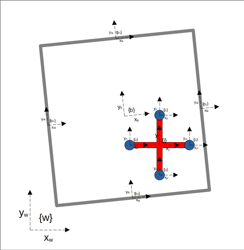
By the way, I’m calling the little rod extending from the center of the jack including the ball on the edge a “prong”.
Top Level Frames
- {\(w\)}: stationary world frame.
- {\(b\)}: the boxes frame.
- {\(j\)}: the jack’s frame.
Subframes
- {\(j_1\)}: child of the {j} frame, residing at the center of the 1st prong.
- {\(j_2\)}: child of the {j} frame, residing at the center of the 2nd prong.
- {\(j_3\)}: child of the {j} frame, residing at the center of the 3rd prong.
-
{\(j_4\)}: child of the {j} frame, residing at the center of the 4th prong.
- {\(b_1\)}: child of the {b} frame, residing at the center of the 1st side of the box.
- {\(b_2\)}: child of the {b} frame, residing at the center of the 2nd side of the box.
- {\(b_3\)}: child of the {b} frame, residing at the center of the 3rd side of the box.
- {\(b_4\)}: child of the {b} frame, residing at the center of the 4th side of the box.
Defining Relationships Between Frames
Now that we’ve defined all of the coordinate frames in the system, we must establish transformation (rotation and position) matricies between all frames with important relationships. It’ll be important to know transformations between the world frame and the box, jack, and all subframes. Additionally, we must know the transformation between all subframes in the jack and all subframes in the box (16 total) in order to calculate the impact equations later on.
Even though we’re working with a planar system, in order to compute kinetic energy from both translation and rotation we need to model the system in the 3D world. The z coordinate will always be zero and all rotation will always be around the z axis.
Transforms from {\(w\)} to {\(b\)} and {\(j\)}
\[g_{wb} = \begin{bmatrix} \cos(\theta_b) & \sin(\theta_b) & 0 & x_b \\ \sin(\theta_b) & \cos(\theta_b) & 0 & y_b \\ 0 & 0 & 1 & 0 \\ 0 & 0 & 0 & 1 \\ \end{bmatrix} \hskip 2em g_{wj} = \begin{bmatrix} \cos(\theta_j) & \sin(\theta_j) & 0 & x_j \\ \sin(\theta_j) & \cos(\theta_j) & 0 & y_j \\ 0 & 0 & 1 & 0 \\ 0 & 0 & 0 & 1 \\ \end{bmatrix}\]Transforms from {\(b\)} to {\(b_1\)}, {\(b_2\)}, {\(b_3\)}, and {\(b_4\)}
\[g_{b1} = \begin{bmatrix} 1 & 0 & 0 & 0 \\ 0 & 1 & 0 & L_b/2 \\ 0 & 0 & 1 & 0 \\ 0 & 0 & 0 & 1 \\ \end{bmatrix} \hskip 2em g_{b2} = \begin{bmatrix} 1 & 0 & 0 & L_b/2 \\ 0 & 1 & 0 & 0 \\ 0 & 0 & 1 & 0 \\ 0 & 0 & 0 & 1 \\ \end{bmatrix}\] \[g_{b3} = \begin{bmatrix} 1 & 0 & 0 & 0 \\ 0 & 1 & 0 & -L_b/2 \\ 0 & 0 & 1 & 0 \\ 0 & 0 & 0 & 1 \\ \end{bmatrix} \hskip 2em g_{b4} = \begin{bmatrix} 1 & 0 & 0 & -L_b/2 \\ 0 & 1 & 0 & 0 \\ 0 & 0 & 1 & 0 \\ 0 & 0 & 0 & 1 \\ \end{bmatrix}\]Transforms from {\(j\)} to {\(j_1\)}, {\(j_2\)}, {\(j_3\)}, and {\(j_4\)}
\[g_{jj1} = \begin{bmatrix} 1 & 0 & 0 & 0 \\ 0 & 1 & 0 & L_j \\ 0 & 0 & 1 & 0 \\ 0 & 0 & 0 & 1 \\ \end{bmatrix} \hskip 2em g_{jj2} = \begin{bmatrix} 1 & 0 & 0 & L_j \\ 0 & 1 & 0 & 0 \\ 0 & 0 & 1 & 0 \\ 0 & 0 & 0 & 1 \\ \end{bmatrix}\] \[g_{jj3} = \begin{bmatrix} 1 & 0 & 0 & 0 \\ 0 & 1 & 0 & -L_j \\ 0 & 0 & 1 & 0 \\ 0 & 0 & 0 & 1 \\ \end{bmatrix} \hskip 2em g_{jj4} = \begin{bmatrix} 1 & 0 & 0 & -L_j \\ 0 & 1 & 0 & 0 \\ 0 & 0 & 1 & 0 \\ 0 & 0 & 0 & 1 \\ \end{bmatrix}\]Transforms from {\(w\)} to {\(b_1\)}, {\(b_2\)}, {\(b_3\)}, {\(b_4\)}, {\(j_1\)}, {\(j_2\)}, {\(j_3\)}, and {\(j_4\)}
\[\begin{align*} g_{wb1} = g_{wb} \cdot g_{bb1} & \hskip 2em g_{wj1} = g_{wj} \cdot g_{jj1} \\ g_{wb2} = g_{wb} \cdot g_{bb2} & \hskip 2em g_{wj2} = g_{wj} \cdot g_{jj2} \\ g_{wb3} = g_{wb} \cdot g_{bb3} & \hskip 2em g_{wj3} = g_{wj} \cdot g_{jj3} \\ g_{wb4} = g_{wb} \cdot g_{bb4} & \hskip 2em g_{wj4} = g_{wj} \cdot g_{jj4} \end{align*}\]Transforms from each side of the box to each prong of the jack
\[\begin{align*} g_{b1j1} = (g_{wb1})^{-1} \cdot g_{wj1} \hskip 2em g_{b2j1} = (g_{wb2})^{-1} \cdot g_{wj1} \\ g_{b1j2} = (g_{wb1})^{-1} \cdot g_{wj2} \hskip 2em g_{b2j2} = (g_{wb2})^{-1} \cdot g_{wj2} \\ g_{b1j3} = (g_{wb1})^{-1} \cdot g_{wj3} \hskip 2em g_{b2j3} = (g_{wb2})^{-1} \cdot g_{wj3} \\ g_{b1j4} = (g_{wb1})^{-1} \cdot g_{wj4} \hskip 2em g_{b2j4} = (g_{wb2})^{-1} \cdot g_{wj4} \\ \\ g_{b3j1} = (g_{wb3})^{-1} \cdot g_{wj1} \hskip 2em g_{b4j1} = (g_{wb4})^{-1} \cdot g_{wj1} \\ g_{b3j2} = (g_{wb3})^{-1} \cdot g_{wj2} \hskip 2em g_{b4j2} = (g_{wb4})^{-1} \cdot g_{wj2} \\ g_{b3j3} = (g_{wb3})^{-1} \cdot g_{wj3} \hskip 2em g_{b4j3} = (g_{wb4})^{-1} \cdot g_{wj3} \\ g_{b3j4} = (g_{wb3})^{-1} \cdot g_{wj4} \hskip 2em g_{b4j4} = (g_{wb4})^{-1} \cdot g_{wj4} \\ \end{align*}\]Constructing the Euler Lagrange Equation
Now that we’ve defined all the transforms we’ll need to simulate the system, it’s time to construct the Euler Lagrange equation.
The first thing we need to do is find the kinetic energy. The equation we’ll use is:
\[KE = \frac{1}{2} (V^b)^T \begin{bmatrix} mI_{n x n} & 0 \\ 0 & \mathcal{I} \end{bmatrix} V^b\]The derivation for this equation is quite long, so I won’t include it here.
Calcuating Body Velocities
A key component of this equation for kinetic energy is \(V^b\). This is the body velocity. The equation for the body velocity in special euclidean (SE(n)) is:
\[\hat{V^b} = g^{-1}\dot{g} = \begin{bmatrix} R & p \\ 0 & 1 \end{bmatrix}^{-1} \begin{bmatrix} \dot{R} & \dot{p} \\ 0 & 0 \end{bmatrix}\]Note, \(V^b\) is hatted.
Even though the jack is made up of four point masses, because its center of mass is at its geometric centroid we can essentially treat it like a single point mass located at the center of the jack with mass equal to \(m_j\) * 4.
This means we’ll need to calculate one body velocity for the jack, and four body velocities for the box.
Unfortunately this equation for the body velocity leaves us with a 4x4 matrix, and the matrix \(\begin{bmatrix} mI_{n x n} & 0 \\ 0 & \mathcal{I} \end{bmatrix}\) is a 6x6. In order to multiply them together, we need to unhat \(V_b\) and turn it into a 6x1 matrix.
\[\begin{gather*} V_j^b = ((g_{wj})^{-1} \cdot \dot g_{wj}) \hskip 0.25em \check{ } \\ V_{b1}^b = ((g_{wb1})^{-1} \cdot \dot g_{wb1}) \hskip 0.25em \check{ } \\ V_{b2}^b = ((g_{wb2})^{-1} \cdot \dot g_{wb2}) \hskip 0.25em \check{ } \\ V_{b3}^b = ((g_{wb3})^{-1} \cdot \dot g_{wb3}) \hskip 0.25em \check{ } \\ V_{b4}^b = ((g_{wb4})^{-1} \cdot \dot g_{wb4}) \hskip 0.25em \check{ } \\ \end{gather*}\]Calculating Inertia Matrices
The final thing we have to do before calculating the kinetic energy is defining the \(I\) matrix, or the inertia matrix, for the box and the jack.
Because the center of mass is at the geometric centroid for both the box and the jack, and there’s no rotation about the x or y axes, the inertia matrix for both look very similar:
\[I_b = \begin{bmatrix} 0 & 0 & 0 \\ 0 & 0 & 0 \\ 0 & 0 & J_b \\ \end{bmatrix} \hskip 2em I_j = \begin{bmatrix} 0 & 0 & 0 \\ 0 & 0 & 0 \\ 0 & 0 & J_b \\ \end{bmatrix}\]Calculating the Total Kinetic Energy of the System
To calculate the total kinetic energy of the system, we can add together the separate kinetic energies of each side of the box, and the total kinetic energy of the jack:
\[\begin{gather} \begin{split} KE_{total} = &\frac{1}{2} ((V^b_{j}\hskip0.1em)^T \begin{bmatrix} mI_{n x n} & 0 \\ 0 & \mathcal{I} \end{bmatrix} V^b_{j} + (V^b_{b1}\hskip0.1em)^T \begin{bmatrix} mI_{n x n} & 0 \\ 0 & \mathcal{I} \end{bmatrix} V^b_{b1} + \\ &(V^b_{b2}\hskip0.1em)^T \begin{bmatrix} mI_{n x n} & 0 \\ 0 & \mathcal{I} \end{bmatrix} V^b_{b2} + (V^b_{b3}\hskip0.1em)^T \begin{bmatrix} mI_{n x n} & 0 \\ 0 & \mathcal{I} \end{bmatrix} V^b_{b3} + \\ &(V^b_{b4}\hskip0.1em)^T \begin{bmatrix} mI_{n x n} & 0 \\ 0 & \mathcal{I} \end{bmatrix} V^b_{b4}) \end{split} \end{gather}\]Calculating the Total Potential Energy of the System
Calculating the total potential energy of the system is relatively easy. We use the normal equation, \(V = mgh\), for each side of the box and the jack as a whole and then we add it all up.
\[V_{total} = g \cdot (4m_jy_j + \frac{m_b}{4} (y_{b1} + y_{b2} + y_{b3} + y_{b4}))\]The y positions of each of the sides of the box can be obtained from the second row, fourth column of the transformation matrices \(g_{wb1}\), \(g_{wb2}\), \(g_{wb3}\), \(g_{wb4}\).
Construct the Lagrangian
The equation for the lagrangian is simple:
\[L = KE_{total} - V_{total}\]Construct the Euler-Lagrange Equation
The Euler-Lagrange Equation is calculated from:
\[\frac{\partial}{\partial t}\frac{\partial L}{\partial \dot q} - \frac{\partial L}{\partial q} = 0\]The right hand side of the equation is zero for now, but next we’ll add in some external forces that will change this.
Adding External Forces
Right now, the box and the jack would just fall downwards at the exact same speed. That’s not very exciting. Let’s add external forces to the box so that it stays in place, and also rotates a bit.
\[F = \begin{bmatrix} 0 \\ F_y \\ \tau_b \\ 0 \\ 0 \\ 0 \end{bmatrix}\]Now, the full Euler-Lagrange equation we’ve created is:
\[\frac{\partial}{\partial t}\frac{\partial L}{\partial \dot q} - \frac{\partial L}{\partial q} = \begin{bmatrix} 0 \\ F_y \\ \tau_b \\ 0 \\ 0 \\ 0 \end{bmatrix}\]Solving the Euler-Lagrange Equations
In software, I substituted in all of our variables and equations with:
- \(L_b = 1\)
- \(L_j = 1\)
- \(m_b = 100\)
- \(m_j = 1\)
- \(J_b = 1\)
- \(J_j = 1\)
- \(g = 9.81\)
and after solving for the accelerations of all configuration variables, I ended up with the following solutions:
\[\begin{gather} \begin{split} &\frac{\partial^2}{\partial t}\theta_b(t) = 0.0623..., \frac{\partial^2}{\partial t}\theta_j(t) = 0.0, \frac{\partial^2}{\partial t}x_b(t) = 0.0, \\ &\frac{\partial^2}{\partial t}x_j(t) = 0.0, \frac{\partial^2}{\partial t}y_b(t) = 0.0, \frac{\partial^2}{\partial t}y_j(t) = -2.453 \end{split} \end{gather}\]And it looks like we have exactly what we want. The box will be rotating, but not falling since it’s acceleration in the y direction is 0. The jack will be falling, and getting knocked around by the block since it’s acceleration in the y direction is non-zero.
These are the Equations of Motion!
Defining the Impact Equations
Defining Constraint Equations
The first thing we need to do is define some constraints.
A constraint equation is represented by the variable \(\phi\). There will be sixteen constraint equations, each one describing a potential collision between a prong of the jack and a wall of the box.
All of the constraint equations will be in this form:
\[\phi_{b_1j_1} = y_{b_1j_1}\]This equation is saying “when the y position of the origin of {\(j_1\)} is 0 relative to the y axis of the {\(b_1\)} frame, an impact has occurred.”
We can create equations just like this for the rest of the possible impacts, and create a 16x1 matrix from them:
\[\phi_{matrix} = \begin{bmatrix} \phi_{b_1j_1} \\ \phi_{b_1j_2} \\ \phi_{b_1j_3} \\ \phi_{b_1j_4} \\ \phi_{b_2j_1} \\ \phi_{b_2j_2} \\ \phi_{b_2j_3} \\ \phi_{b_2j_4} \\ \phi_{b_3j_1} \\ \phi_{b_3j_2} \\ \phi_{b_3j_3} \\ \phi_{b_3j_4} \\ \phi_{b_4j_1} \\ \phi_{b_4j_2} \\ \phi_{b_4j_3} \\ \phi_{b_4j_4} \end{bmatrix}\]Creating the impact equations
There are two equations that make up what I’ve been calling the “impact equations”:
\[\begin{gather} \frac{\partial L}{\partial \dot q}\Bigg|_{\tau^-}^{\tau^+} = \lambda\frac{\partial \phi}{\partial q} \\ \\ \Bigg[\frac{\partial L}{\partial \dot q} \cdot \dot q - L(q,\dot q)\Bigg] \Bigg|_{\tau^-}^{\tau^+} = 0 \end{gather}\]\(\tau^-\) and \(\tau^+\) represent the time immediately before impact occurs and the time immediately after impact occurs, respectively.
The first equation can be interpreted as restricting the change in momentum due to impact to lie perpendicular to the contact surface. The second equation states that the Hamiltonian (which is the total energy in the system, in most cases) is conserved through the impact.
After the impact equations are fully constructed, we’re going to end up with 112 possible equations (16 impact conditions, each with 7 equations).
As we simulate the jack and box, we’ll be checking if any of the impact conditions are met every iteration. If one is met, then we’ll use the 7 equations associated with that impact condition to solve for \(\dot q(\tau^+)\).
Solving for the velocity of all configuration variables at the moment just after impact allows us to accurately update the jack’s and box’s trajectory and create a realistic simulation.
There’s no need to solve for \(q(\tau^+)\), since it’s the exact same as \(q(\tau^-)\), which is known.
Simulating the System
Finally everything is in place for us to simulate the system.
We start by defining a threshold that determines when an impact occurs. After some trial and error, I chose 0.3 meters. Each iteration of the simulation, we check to see if any of our 16 impact conditions have been met. To do this, we can use sympy lambdify to make our \(\phi_{matrix}\) into an executable function.
The function to check if an impact has occurred is quite simple, so I’ll include it below for better understanding:
def impact_condition(s, thresh):
    """
    Check if an impact has occurred.

    Check if an impact has occured and if it has
    return True, and where in the phi matrix it
    occurred.

    Args:
    ----
    s: The current configuration variables.
    thresh: The threshold for impact to have occurred.

    Returns:
    -------
    bool: Whether or not an impact occurred.
    i: Which impact condition was triggered.

    """
    phiq = phi_mat_lam(*s)
    for i,phi in enumerate(phiq):
    if phi < thresh and phi > -thresh:
        return True, i
    return False, i
”s” takes the form:
\[s = \begin{bmatrix} x_b & y_b & \theta_b & x_j & y_j & \theta_j & \dot x_b & \dot y_b & \dot \theta_b & \dot x_j & \dot y_j & \dot \theta_j \end{bmatrix}\]If an impact has occurred, we need to access the 7 equations associated with this impact condition and plug in the configuration variables at the current time step.
Next, we solve these 7 equations for lambda and \(\dot q(\tau^+)\). We’ll get two solutions for lambda, and each solution for lambda has a unique \(\dot q(\tau^+)\). We only want the solution with a positive value for lambda. The reason for this is that the wall can only act away from its surface, and a negative lambda would correspond to the wall sucking the point in.
What is lambda? As far as I understand, it’s a scalar value corresponding to the magnitude of the force required to enforce a constraint.
Once we have \(\dot q(\tau^+)\), we can substitute it in for the configuration variables’ velocities at the current time step (final six variables in the s matrix).
Once the simulation concludes, then all we have to do is animate it. The code for animating the system is repetitive, and I’ll leave it as an exercise for the reader to go and checkout my github to see how it works.
The gif at the top shows an example of the animated simulation, but here it is again:
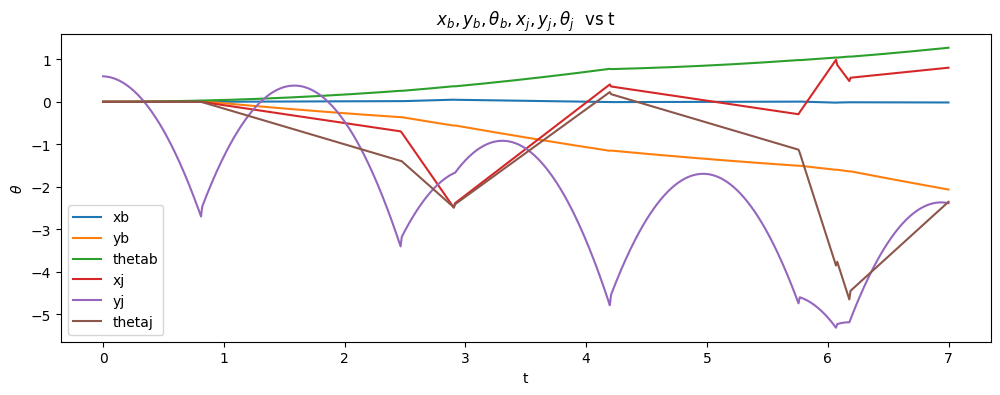
And here’s a graph of all configuration variables during the simulation time: