Rapidly-Exploring Random Tree (RRT) Path Planning
This project implements the rapidly-expanding random tree algorithm, first developed by Steven LaValle in 1988.
A link to his original paper is here.
Link to this project’s Github
How to Run
To run the file, navigate to the directory where the script is stored and run:
$ python rrt.py
The file has two modes:
- Mode 0: The only obstacle is the Northwestern “N”
- Mode 1: There are many circular obstacles. The default is 20 circles.
You can also specify arguments that allow you to change modes, or determine the number of obstacles.
usage: rrt.py [-h] [-m] [-o]

Process arguments to decide the type of obstacle the RRT algorithm will have to search around, and
in some cases the number of obstacles.

options:
  -h, --help         show this help message and exit
  -m , --mode        an integer to define the mode
  -o , --obstacles   an integer to define the number of obstacles
Here’s an example with the arguments:
$ python rrt.py -m 1 -o 40
Implementation
Background
A Rapidly-Exploring Random Tree (RRT) is a fundamental path planning algorithm in robotics.
An RRT consists of a set of vertices, which represent configurations in some domain D and edges, which connect two vertices. The algorithm randomly builds a tree in such a way that as the number of vertices n increases to \( \infty \), the vertices are uniformly distributed across the domain \(D \subset R^n \).
The algorithm, as presented below, has been simplified from the original version by assuming a robot with dynamics \( \dot{q} = u \) where \(\lVert u \rVert = 1 \) and assuming that we integrate the robot’s position forward for \(\Delta{t} = 1 \).
Overview
Here is some pseudocode that generally represents the RRT algorithm:
Input: \(q_{init} \leftarrow\) The initial node \(q_{goal} \leftarrow\) The known position of the goal \(K \leftarrow\) The number of nodes in RRT \(\Delta \leftarrow\) Incremental distance \(D \leftarrow\) The planning domain Output: \(G \leftarrow\) the RRT
Algorithm: Initialize \(G\) with \(q_{init}\) Initialize obstacle(s) with \(q_{init}\) repeat \(K\) times \(q_{rand} \leftarrow\) RANDOM_CONFIGURATION(D) \(q_{near} \leftarrow\) NEAREST_VERTEX(\(q_{rand}, G\)) \(q_{new} \leftarrow\) NEW_CONFIGURATION(\(q_{near}, q_{rand}, \Delta\)) Check if \(q_{new}\) collides with an obstacle Add vertex \(q_{new}\) to \(G\) Add an edge between \(q_{near}\) and \(q_{new}\) in \(G\) Check if \(q_{new}\) can see the goal end repeat return \(G\)
Results
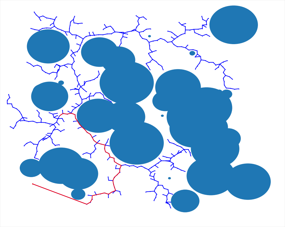
Running the python script will spawn a window generated by matplotlib, and the algorithm will immediately start executing. Nodes of the tree appear as blue dots, and the lines connecting the nodes are also blue. Obstacles appear black, and the goal node appears as red.
If the position of the newest node has a clear line of sight to the goal node, the algorithm will draw a straight line from the new node to the goal node. Next, the function will return G, which will be a dictionary of all of the parent child relationships of all the nodes in the RRT.
Using G, we can construct the shortest path from the initial position to the goal position. The code draws this path in red once it has found the goal.
Here is an image of what the algorithm looks like after it has finished executing using mode 0:

And here is an image of what the algorithm looks like after it has finished executing mode 1: